
Interactive Data Graphics Analyzing Global Temperatures Over the Years
In this blog post, I will create three interesting, interactive data graphics using the NOAA climate data.
Each interactive data graphic will address three key questions:
- How does the average yearly change in temperature vary within a given country?
- How does the change in average temperatures vary between different countries over a certain amount of years?
- How do temperature trends of a country compare to other countries during a specific month over a certain amount of years?
§1. Create a Data Base
Here I will create a database with three tables: temperatures, stations, and countries.
Importing Data
First you need to import the following packages by running the following code:
import pandas as pd
import sqlite3
import numpy as np
from sklearn.linear_model import LinearRegression
from matplotlib import pyplot as plt
from plotly import express as px
import calendar
You are probably familiar with pandas, numpy, sklearn, matplotlib, and calendar. Here we will also be importing sqlite3 (allows us to work with databases) and plotly (helps create interactive graphics).
Reading the Data into Python
Then you need to read the data from each of the three tables by running the following code:
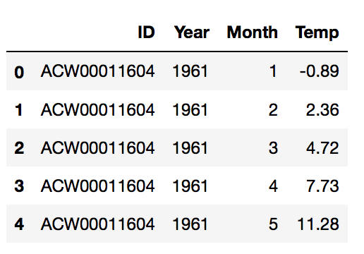
temps = pd.read_csv("temps_stacked.csv")
temps.head()
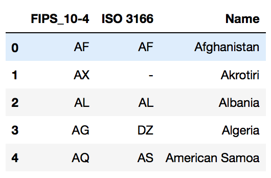
countries = pd.read_csv('countries.csv')
Since whitespaces in column names are bad for SQL, we will run the following code:
countries = countries.rename(columns= {"FIPS 10-4": "FIPS_10-4"})
countries.head()
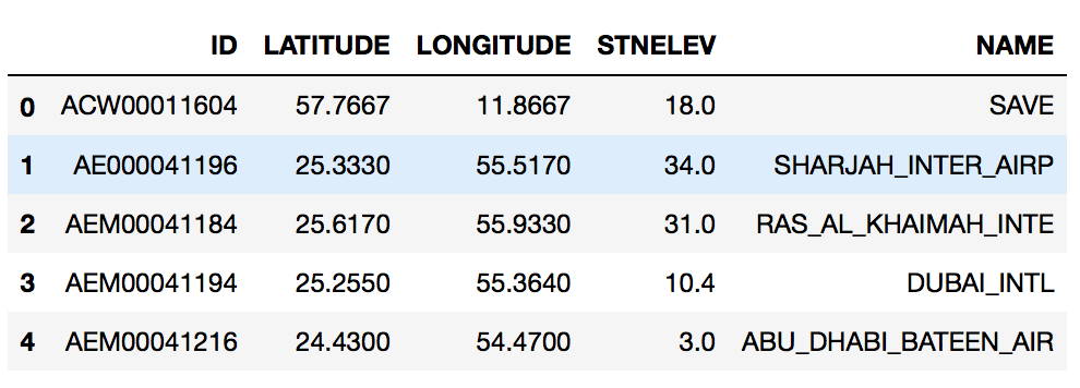
stations = pd.read_csv('station-metadata.csv')
stations.head()
Create Database
Now, we will open a connection to temps.db so that you can ‘talk’ to it using python and create a database with three tables; temperatures, countries, stations. Then always remember to close the connection after.
conn = sqlite3.connect("temps.db")
temps.to_sql("temperatures", conn, if_exists="replace", index=False)
countries.to_sql("countries", conn, if_exists="replace", index=False)
stations.to_sql("stations", conn, if_exists="replace", index=False)
# always close your connection
conn.close()
§2. Write a Query Function
Next, we will write a Python function called query_climate_database() which accepts four arguments:
- country, a string giving the name of a country (e.g. ‘South Korea’) for which data should be returned.
- year_begin and year_end, two integers giving the earliest and latest years for which should be returned.
- month, an integer giving the month of the year for which should be returned.
The return value of query_climate_database() is a Pandas dataframe of temperature readings for the specified country, in the specified date range, in the specified month of the year.
def query_climate_database(country, year_begin, year_end, month):
"""
To Return:
Pandas dataframe of temperature readings for the specified country,
in the specified date range, in the specified month of the year.
"""
#connect to database
conn = sqlite3.connect("temps.db")
#SQL QUERY
cmd = \
f"""
SELECT S.name, S.latitude, S.longitude, C.name Country, T.year, T.month, T.temp
FROM countries C
LEFT JOIN stations S ON SUBSTRING(S.id, 1, 2) = C."FIPS_10-4"
LEFT JOIN temperatures T ON T.id = S.id
WHERE (C.name = "{country}") AND (T.year BETWEEN {year_begin} AND {year_end}) AND (T.month = {month})
"""
#convert to dataframe
df = pd.read_sql_query(cmd, conn)
conn.close()
return df
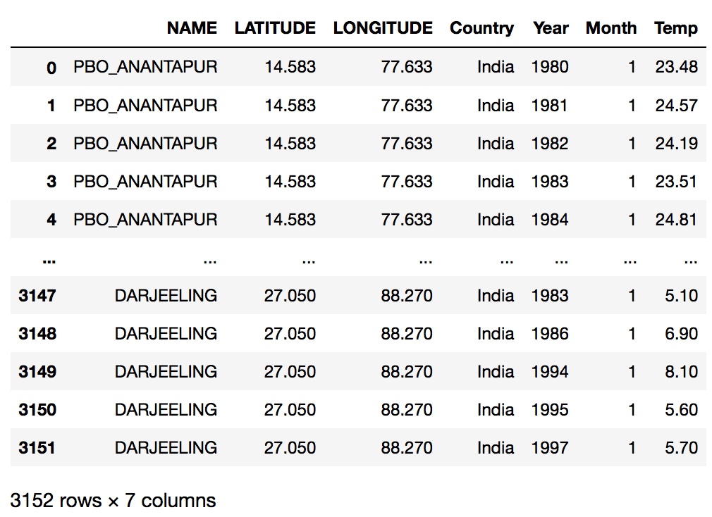
Next we will test our Query function by running the following code:
query_climate_database(country = "India",
year_begin = 1980,
year_end = 2020,
month = 1)
§3. Write a Geographic Scatter Function for Yearly Temperature Increases
For our first interactive graphic we will be adressing the question;
How does the average yearly change in temperature vary within a given country?
Next we will write a function called temperature_coefficient_plot(). This function will accept five explicit arguments, and an undetermined number of keyword arguments.
- country, year_begin, year_end, and month should be as in the previous part.
- min_obs, the minimum required number of years of data for any given station. Only data for stations with at least min_obs years worth of data in the specified month should be plotted; the others should be filtered out. df.transform() plus filtering is a good way to achieve this task.
- **kwargs, additional keyword arguments passed to px.scatter_mapbox(). These can be used to control the colormap used, the mapbox style, etc.
The output of this function should be an interactive geographic scatterplot, constructed using Plotly Express, with a point for each station, such that the color of the point reflects an estimate of the yearly change in temperature during the specified month and time period at that station.
First we will compute the first coefficient of a linear regression model.
def coef(data_group):
X = data_group[["Year"]]
y = data_group["Temp"]
LR = LinearRegression()
LR.fit(X, y)
slope = LR.coef_[0].round(4)
return slope
Next we will write the function called temperature_coefficient_plot() by running the following code:
def temperature_coefficient_plot(country, year_begin, year_end, month, min_obs, **kwargs):
'''
The output of this function is an interactive geographic scatterplot with a point for each station,
such that the color of the point reflects an estimate of the yearly change in temperature during
the specified month and time period at that station.
'''
#Get a dataframe to plot data
df = query_climate_database(country, year_begin, year_end, month)
#filter data to only plot stations with at least min_obs years worth of data in the specified month
num_obs = df.groupby("NAME")["Year"].transform(len)
df["num_obs"] = num_obs.to_frame()
df = df[df["num_obs"] >= min_obs]
#Apply Linear regression to get the increase coefficient
coefs = df.groupby(["NAME", "LATITUDE", "LONGITUDE", "Country"]).apply(coef)
coefs = coefs.reset_index()
coefs = coefs.rename(columns = {0 : "Estimated Yearly Increase (°C)"})
#plot the scatterplot
fig = px.scatter_mapbox(coefs,
lat = "LATITUDE",
lon = "LONGITUDE",
hover_name = "NAME",
color = "Estimated Yearly Increase (°C)",
color_continuous_midpoint = 0,
title = \
f"""
Estimates of yearly increase in temperature in {calendar.month_name[month]}
<br>for stations in {country}, years {year_begin} - {year_end}""",
**kwargs)
return fig
After writing the function, you should be able to create a plot of estimated yearly increases in temperature during the month of January, in the interval 1980-2020, in India, as follows:
# assumes you have imported necessary packages
color_map = px.colors.diverging.RdGy_r # choose a colormap
fig = temperature_coefficient_plot("India", 1980, 2020, 1,
min_obs = 10,
zoom = 2,
mapbox_style="carto-positron",
color_continuous_scale=color_map)
fig.show()
Let’s look at another interactive geographic scatterplot for Australia between the years 1990 to 2010 in the month of July.
# assumes you have imported necessary packages
color_map = px.colors.diverging.RdGy_r # choose a colormap
fig = temperature_coefficient_plot("Australia", 1990, 2010, 7,
min_obs = 10,
zoom = 2,
mapbox_style="carto-positron",
color_continuous_scale=color_map)
fig.show()
In both these plot, we are able to hover over the data points and see the station name, latitude and longitude coordinates, and the estimated yearly increase (°C).
Choropleth Map
For our second interactive graphic we will be adressing the question;
How does the change in average temperatures vary between different countries over a certain amount of years?
We will be creating a Choropleth map in order to explore this question.
First we need a GeoJSON file containing the coordinates for the country polygons. The code below uses the json module to read a GeoJSON file from the web. This file contains the borders of countries.
from urllib.request import urlopen
import json
countries_gj_url = "https://raw.githubusercontent.com/PhilChodrow/PIC16B/master/datasets/countries.geojson"
with urlopen(countries_gj_url) as response:
countries_gj = json.load(response)
Now we need a data frame containing the temperature variation between our start and end year for each country.
def query_climate_database2(year_begin, year_end):
"""
To Return:
Pandas dataframe of yearly average temperatures for the specified country,
in the specified year range.
"""
#reconnect to database
conn = sqlite3.connect("temps.db")
#SQL QUERY
cmd = \
f"""
SELECT C.name Country, T.year, AVG(T.temp) mean_temp
FROM countries C
LEFT JOIN temperatures T ON SUBSTRING(T.id, 1, 2) = C."FIPS_10-4"
WHERE T.year BETWEEN {year_begin} AND {year_end}
GROUP BY T.year, C.name
"""
#convert to data frame
df = pd.read_sql_query(cmd, conn)
conn.close()
return df
Now, we’ll write a function called avgtemp_variation(). This function will accept two explicit arguments, and an undetermined number of keyword arguments.
- year_begin / year_end, two integers giving the earliest and latest years for which should be returned.
- kwargs, additional keyword arguments passed to px.choropleth(). These can be used to control the colormap used, the mapbox style, etc.
def avgtemp_variation(year_begin, year_end, **kwargs):
"""
The output of this function is a choropleth map showing
the variation of average temperatures between different countries
in the specified year range.
"""
#Get a dataframe to plot data
df = query_climate_database2(year_begin, year_end)
#create a pivot table so the cols = years, index = countries, vals = mean_temp
df = pd.pivot(df, index = "Country", columns = "Year", values = "mean_temp")
df= df.reset_index()
#add temp variation column
df["Variation (°C)"] = (df[year_end] - df[year_begin]).round(2)
#clean dataframe
df = df[["Country", "Variation (°C)"]].groupby("Country").mean()
df = df.reset_index()
#plot choropleth
fig = px.choropleth(df,
geojson = countries_gj,
locations = "Country",
locationmode = "country names",
color="Variation (°C)",
scope="world",
height=300,
title = \
f"""
Average temperature change by country from {year_begin} - {year_end}""",
**kwargs)
fig.update_layout(margin={"r":0,"t":30,"l":0,"b":0})
return fig
Let’s test our map between the years 1980 to 2020.
fig = avgtemp_variation(1980, 2020)
fig.show()
In this map, we are able to hover over the different countries and see the country name and how much the average temperature of the country has varied/changed (°C) between 1980 to 2020.
Box Plot
For our third interactive graphic we will be adressing the question;
How do temperature trends of a country compare to other countries during a specific month over a certain amount of years?
Next we will write a function called temp_trends(). This function will accept four explicit arguments, and an undetermined number of keyword arguments.
- country, year_begin, year_end, and month should be as in the previous part.
- **kwargs, additional keyword arguments passed to px.scatter_mapbox(). These can be used to control the colormap used, the mapbox style, etc.
def temp_trends(country, year_begin, year_end, month, **kwargs):
df_con = []
for i in country:
df = query_climate_database(i, year_begin, year_end, month)
df_con.append(df)
#concatenate all query results into one df
df = pd.concat(df_con)
countries = ", ".join(country)
#plot boxplot
fig = px.box(df,
x = "Year",
y = "Temp",
facet_row = "Country",
color = "Country",
hover_name = "Year",
title = \
f"""
Temperature trends in {calendar.month_name[month]} for {countries},
<br> years {year_begin} - {year_end}""",
**kwargs)
return fig
Let’s test our plot comparing the countries India, Australia, and France between the years 1990 to 2010 in the month of June.
fig = temp_trends(["India", "Australia", "France"], 1990, 2010, 6)
fig.show()
In this plot, we are able to hover over the data points and see the year, country name and average monthly temperature for June. The plot is dividing into three different plots, one for each country and color coded. We are able to clearly compare the temperatures trends between the countries, India, Australia, and France.